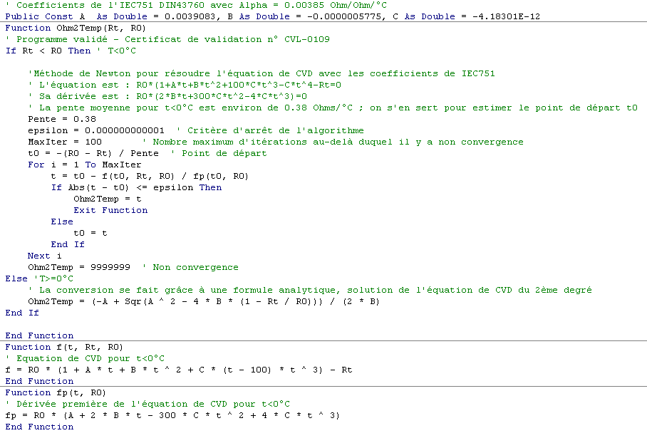
The CVD equation calculates resistance as a function of temperature; this is the converse of the most common applications: temperature as a function of resistance. In order to convert the RTD resistance into temperature, we need to use a 2nd degree quadratic equation, which is in a sense the reciprocal of the CVD equation but only for temperatures above 0°C:
$$ T = \frac{{ – A + \sqrt {{A^2} – 4B\left( {1 – \frac{{{R_T}}}{{{R_0}}}} \right)} }}{{2B}} $$
For temperatures below 0°C, the CVD equation is too complex to solve, and it is necessary to use numerical methods. The most accurate is to find the root of the CVD equation numerically; in other words, to solve the following equation:
$$ f\left( T \right) = {R_0}\left[ {1 + AT + B{T^2} + C\left( {T – 100} \right){T^3}} \right] – {R_T} = 0 $$
The most appropriate method is the tangent method (or Newton’s algorithm). This method has the advantage of converging with certainty provided that the root is within the given interval, which is achievable knowing the average sensitivity of an RTD. This method also requires knowing the derivative of the CVD equation which can easily be calculated:
$$ \frac{{df\left( T \right)}}{{dT}} = {R_0}\left[ {A + 2BT + 4C{T^3} – 300C{T^2}} \right] $$
Finally, it is necessary to be certain that the equation has only one root, which is the case with the CVD equation. The algorithm, simple, can be found in all books on numerical methods. It consists in determining for a starting point $$ {{t_0}} $$, the tangent at this point $$ f’\left( {{t_0}} \right) $$ which intersects with the curve at a new point $$ {{t_1}} $$. At this point, we recalculate the tangent $$ f’\left( {{t_1}} \right) $$ which in turn intersects with the curve at a point $$ {{t_2}} $$, etc… until the gap between two successive points is smaller than the stopping criterion (defined by ε). The program “RTD.xls” uses this algorithm. Here is the source code:


