Frequently Asked Questions
50 Frequently Asked Questions About Thermocouples
Temperature is not a quantity in the strict sense of the term as the majority of other measurement units are. A quantity is something which can be increased or decreased, for example length, area, power output, etc.
Measuring a quantity G (of whatever nature) means comparing it to another quantity U of the same nature, chosen as the unit. The result of the measurement is a whole number (for example 5) if the unit U is contained a whole number of times in the quantity G in question (5 times in this case). A quantity is directly measurable if we can define the relationship or the equality or the sum of two values of such quantity. Length and area are measurable quantities.
On the other hand, a temperature referenced using the Celsius temperature scale is not a measurable quantity; we can identify the equality of two temperatures but we cannot add them. You can therefore refer to: evaluating, comparing, marking or indicating temperatures but not measuring them in the correct sense of the term.
There are currently two units of temperature in the International System:
Kelvin, symbol K
Degree on the thermodynamic scale of absolute temperatures where the triple point of water is 273.16 K
Degree Celsius, symbol °C
The Celsius temperature t corresponding to the thermodynamic temperature T is defined by the equation t = T – T0 where T0 = 273.15 K
A temperature interval or difference can also be expressed in degrees Celsius. In the past, a number of temperature measurement scales have been defined based on two or more fixed points.
It should be noted that the kelvin is not used with the word degree or the symbol; we say “a kelvin” and not a degree kelvin.
The ITS (International Temperature Scale) uses 17 temperature reference points based on the physical phenomenon of the triple point, the vapour pressure, the freezing point, melting point and solidification point of different substances. These distinct points occur at a fixed, reproducible temperature, determined by nature. They do not require the use of a reference sensor in order to measure them. For example, gallium always melts (goes from solid state to liquid state) at 29.7646°C. A distinct fixed point is the triple point. And a distinct triple point is the triple point of water (0.01°C under 1 atm).
The triple point is the point at which the vaporisation curve, the sublimation curve and the fusion curve of a substance meet. It was Josiah W. Gibbs (1839-1903) who recognised and proposed the phase rule: the three states, solid, liquid, gas, only coexist at one unique point within the thermodynamic parameters, the triple point. Vapour, liquid and solid are found together at a unique defined temperature and pressure.
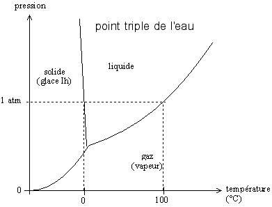
Figure 1. Change in pressure with temperature for the triple point of water
The ITS (International Temperature Scale) uses 17 temperature reference points:
| Element | Symbol | Type | K | °C |
| Helium | He | Vapour pressure | 5 | -268.15 |
| Hydrogen | H2 | Triple point | 13.8033 | -259.3467 |
| Hydrogen | H2 | Vapour pressure | 17 | -256.15 |
| Hydrogen | H2 | Vapour pressure | 20.3 | -252.85 |
| Neon | Ne | Triple point | 24.5561 | -248.5939 |
| Oxygen | O2 | Triple point | 54.3584 | -218.7916 |
| Argon | Ar | Triple point | 83.8058 | -189.3442 |
| Mercury | Hg | Triple point | 234.315 | -38.8344 |
| Water | H2O | Triple point | 273.16 | 0.01 |
| Gallium | Ga | Melting | 302.9146 | 29.7646 |
| Indium | In | Freezing | 429.7485 | 156.5985 |
| Tin | Sn | Freezing | 505.078 | 231.928 |
| Zinc | Zn | Freezing | 692.677 | 419.527 |
| Aluminium | Al | Solidification | 933.473 | 660.323 |
| Silver | Ag | Freezing | 1234.93 | 961.78 |
| Gold | Au | Freezing | 1337.33 | 1064.18 |
| Copper | Cu | Freezing | 1357.77 | 1084.62 |
A current will circulate in a closed circuit comprising two dissimilar conductors if a temperature difference is maintained between the two junctions.

Figure 2 Closed circuit: diagram showing in general terms how a thermocouple works
Broken circuit: heating the junction between the two different metals A and B creates a voltage eAB; it is a function of the temperature at the junction and the composition of the two metals. All dissimilar metals produce this effect.

Figure 3 Open circuit showing in general terms how a thermocouple works
The production of a voltage between dissimilar metals with their ends at different temperatures is a function of the three thermoelectric effects in metals:
- The Seebeck effect: Thomas Johann Seebeck (1770-1831) was the first person to demonstrate the thermoelectric effects of producing currents which occur in a circuit comprising two metals where the two welds are at different temperatures. He did not fail to note the phenomenon caused by a temperature difference along a homogeneous conductor; a phenomenon which would be rediscovered thirty years later by William Thomson and called the Thomson Effect.
- The Peltier effect: Jean Charles Athanase Peltier, French physicist (1785-1845), gave up the profession of watchmaker at the age of thirty to devote himself to experimental physics; he is known for his discovery in 1834 of the Peltier effect: when an electric current passes through the junction of two dissimilar metal conductors, there is a rise or fall in temperature depending on the direction of the current; the amount of heat released or absorbed is proportional to the strength of the current. It is in a sense the converse of the Seebeck effect. Passing a current can therefore cause heat to be absorbed; this effect is used in some small refrigerators or to cool electric circuits.
- The Thomson effect: This was discovered by Lord Kelvin (then Sir William Thomson) – but already noted by Seebeck – who proved its existence by experiment after demonstrating it theoretically. It is a sort of Peltier effect but between contiguous sections of the same metal bar. The Thomson effect relates to the production – or absorption – of heat caused by passing a current through a section of a conductor where there is a difference in temperature between the ends of the section.
The electromotive force (EMF) produced in a thermocouple circuit depends on the nature of the two conductors and the temperatures at the two junctions; these are called respectively:
- Hot junction: Thermocouple junction subjected to the temperature to be measured: the Sensor junction
- Cold junction: Thermocouple junction maintained at a known temperature or at 0 °C: the Reference junction.
There are 8 common types of thermocouples:
| Type | Metal A (+) | Metal B (-) | Theoretical limits | Seebeck coef. α (µV/°C) at T°C | Standard error | Min. error |
| B | Platinum 30% Rhodium | Platinum 6% Rhodium | 0 to 1820°C | 5,96 µv at 600°C | 0,5% | 0,25% |
| E | Nickel 10% Chrome | Constantan | -270 to 1000°C | 58,67 µV at 0°C | 1,7% to 0,5% | 1% to 0,4% |
| J | Iron | Constantan | -210 to 1200°C | 50,38 µV at 0°C | 2,2% to 0,75% | 1,1% to 0,4% |
| K | Chromel | Alumel | -270 to 1372°C | 39,45 µV at 0°C | 2,2% to 0,75% | 1,1% to 0,2% |
| N | Nicrosil | Nisil | -270 to 1300°C | 25,93 µV at 0°C | 2,2% to 0,75% | 1,1% to 0,4% |
| R | Platinum 13% Rhodium | Platinum | -50 to 1768°C | 11,36 µV at 600°C | 1,5% to 0,25% | 0,6% to 0,1% |
| S | Platinum 10% Rhodium | Platinum | -50 to 1768°C | 10,21 µV at 600°C | 1,5% to 0,25% | 0,6% to 0,1% |
| T | Copper | Constantan | -270 to 400°C | 38,75 µV at 0°C | 1% to 0,75% | 0,5% to 0,4% |
The metals and alloys used have proven properties and are standardised at international level in terms of materials, transfer curves, symbols, tolerances and colour codes in accordance with standards:
- IEC 584-1 (formerly NF C 42-321) Reference tables – e = f(Θ)
- IEC 584-2 (formerly NF C 42-322) Tolerances
- IEC 584-3 (formerly NF C 42-323) Identification of thermocouples and compensating cables
- IEC 584-4 (formerly NF C 42-324) Extension and compensating cables for thermocouples
- IEC 584-5 (formerly NF C 42-325) “Coated” cables and thermocouples
| Type | Colours IEC 584-3 (+ / -) | Colours NF C 42-323 1985 (+ / -) | Usage range | Tolerances NF EN 60-584 Class 1 | Tolerances NF EN 60-584 Class 2 |
| B | Grey / White | Yellow / Grey | +600 to +1700°C | – | ±0.0025.Θ from 600 to +1700°C |
| E | Purple / White | Yellow / Orange | -40 at +900°C | ±1.5°C from -40 to +375°C ±0.0004.Θ from 375 to800°C | ±2.5°C from -40 to +333°C ±0.0075.Θ from 333 to 900°C |
| J | Black / White | Yellow / Black | -40 to +750°C | ±1.5°C from -40 to +375°C ±0.004.Θ from 375 to 750°C | ±2.5°C from -40 to +333°C ±0.0075.Θ from 333 to 750°C |
| K | Green / White | Yellow / Purple | -40 to +1200°C | ±1.5°C from -40 to +375°C ±0.004.Θ from 375 to 1000°C | ±2.5°C from -40 to +333°C ±0.0075.Θ from 333 to 1200°C |
| N | Pink / White | – | -40 to +1200°C | ±1.5°C from -40 to +375°C ±0.004.Θ from 375 to 1000°C | ±2.5°C from -40 to +333°C ±0.0075.Θ from 333 to 1000°C |
| R | Orange / White | Yellow / Green | 0 to +1600°C | ±1.0°C from 0 to +1100°C ±1+0.003.(Θ-1100) from 1100 to 1600°C | ±1.5°C from 0 to +600°C ±0.0025.Θ from 600 to 1600°C |
| S | Orange / White | Yellow / Green | 0 to +1600°C | ±1.0°C from 0 to +1100°C ±1+0.003.(Θ-1100) from 1100 to 1600°C | ±1.5°C from 0 to +600°C ±0.0025.Θ from 600 to 1600°C |
| T | Brown / White | Yellow / Blue | -40 to +350°C | ±0.5°C from -40 to +125°C ±0.004.Θ from 125 to 350°C | ±1.0°C from -40 to +133°C ±0.0075.Θ from 133 to 350°C |
Constantan is an alloy of copper and nickel characterised by an electrical resistance virtually independent of temperature and therefore suitable for building electrical resistors. As copper and nickel are two perfectly isomorphous metals, they can be mixed in the liquid state in any proportions. Depending on the proportions of copper and nickel, the conductivity curve of the alloy has a distinctive shape with a very pronounced minimum around the 50% mark and a very rapid increase as it approaches pure metal. In practice, an alloy of 60% copper and 40% nickel is generally used with a specific resistance of 0.5 Ω/mm²/m.
These two metals can also form an alloy by simple diffusion without passing through the liquid phase. The experiment was conducted by Bruni who heated a copper wire on which a layer of nickel had been deposited. The resistance of the ensemble increased very markedly following the formation of constantan. NB: Constantan is the generic name for alloys of copper and nickel whatever the percentages of the two metals. The Constantan used in type T thermocouples (Copper/Constantan) is not the same as that used in type J thermocouples (Iron/Constantan).
Although type B thermocouples have a specified theoretical range from 0 to 1820°C, there is uncertainty and calculations are problematic in the zone between 0 °C and 100 °C where the thermoelectric voltage fluctuates between -0.003 mV and +0.003 mV (0 to 50 °C) then increases very gradually up to 0.033 mV at 100 °C. In order to be able to make calculations with certainty to an accuracy of 1 °C in this zone, a means of measurement with a resolution of at least 0.01 µV for an accuracy of 0.1 µV would be required, but the ITS-90 table gives only an accuracy of 1 µV for type B. The standardised usage range is from +600 to +1700°C. The bottom limits for the calculations will therefore be 100 °C or 0.033 mV.
Type B thermocouples are commonly called: 18% thermocouples (explanation: 30% Rhodium (Positive) + 6% Rhodium (Negative) equals 36% divided by two gives 18%).
There are other types of thermocouples, such those based on Tungsten (W) alloyed with Rhenium (Re) to make it more malleable. They are used for very high temperatures in a vacuum or inert atmosphere. They are type C (W-5%Re/W-26%Re), type D (W-3%Re/W-25%Re) and type G (W/W-26%Re).
In the case of small changes in temperature, the change in voltage is proportional to the change in temperature. The coefficient of proportionality is called the Seebeck coefficient and denoted by the symbol α.
One of the most commonly used thermocouples is the Chromel-Alumel or Type K Thermocouple. It has a wide measurement range (-100 to + 1370 °C), a large electromotive force (41310 µV at 1000 °C with the cold junction at 0°C) and a curve which can be easily linearised to give accuracies better than 0.2% over the entire measurement range. The type K thermocouple is made of Alumel: an alloy comprising 95% nickel, 2% aluminium, 2% manganese and 1% silicon and Chromel an alloy comprising 80% nickel and 20% chromium.
Now that we know that a thermocouple generates a voltage the magnitude of which is a function of the temperature and the Seebeck coefficient (α) of the junction of the two dissimilar metals, all that remains is to measure this using a voltmeter and then calculate the temperature from the voltage measured.
Connection to a voltmeter
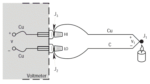
Let’s connect a Copper/Constantan thermocouple (Type T) to the terminals of a voltmeter and making the calculation using α = 38.75µV/°C, we obtain a temperature figure which is independent of the environment around the thermocouple.
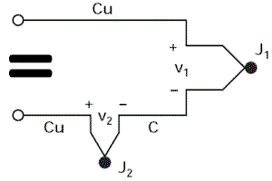
Finally, by referring to the equivalence diagram (=), the resulting voltage measured by the voltmeter is equal to V1 – V2, i.e. It is proportional to the temperature difference between J1 and J2.
We can only find the temperature of J1 if we know that of J2.
Reference to the external junction
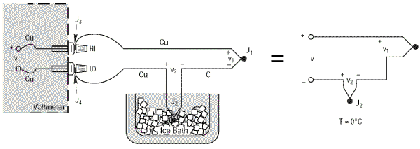
A simple way of the determining the temperature of junction J2 accurately and easily is to immerse it in a bath of melting ice which forces its temperature to 0°C (273.15 K). J2 can then be taken as the reference junction. Thus there is now a reference value of 0°C at J2.
And using a different type of thermocouple?
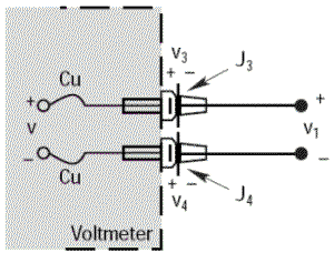
The previous examples used a Copper/Constantan thermocouple (Type T) which is simple to use for demonstrations as the voltmeter terminals are also made of copper and this only induces a single parasitic junction. Let’s go through the same example with an Iron/Constantan thermocouple (Type J) instead of Copper/Constantan.
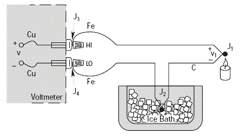
The voltmeter will show a voltage V equal to V1 only if the thermoelectric voltages V3 and V4 are identical, since they are in opposition; i.e. if the parasitic junctions J3 and J4 are at the same temperature.
It is essential that the voltmeter connection terminals are at the same temperature in order to prevent any drift in the measurement.
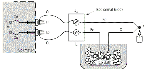
This problem can be eliminated by extending the copper wires so that they are only connected as close as possible to the thermocouple using an isothermal junction block. This type of block is an electrical insulator but a good heat conductor such that it keeps junctions J3 and J4 permanently at an identical temperature. By proceeding thus we can very easily move the thermocouple away from the measuring instrument without causing problems. The temperature of the isothermal block is irrelevant as the thermoelectric voltages at the two Cu-Fe junctions are in opposition.
We will still have: V = α(TJ1 – TREF)
Eliminating the bath of melting ice
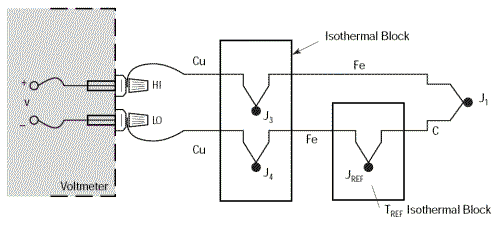
The circuit described above enables us to take accurate, reliable measurements away from the thermocouple, but how useful it would be to eliminate the need for the bath of melting ice. Let’s begin by replacing the bath of melting ice with another isothermal block which will be kept at the temperature TREF.
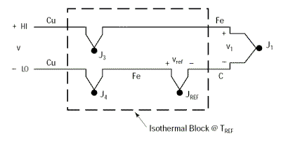
Since we have already seen that the temperature of the isothermal block supporting junctions J3 and J4 is not relevant – provided that these two junctions are at the same temperature – there is no reason not to combine the two blocks into one which will be kept at the temperature TREF.
We will still have: V = α(TJ1 – TREF)

However, this new circuit has the disadvantage that it requires two thermocouples to be connected. We can happily eliminate the additional thermocouple by combining the junctions Cu-Fe (J4) and Fe-C (JREF). This is possible due to the law of intermediate metals. This empirical law states that a third metal (in this case Iron) inserted between the two different metals in a thermocouple does not affect the voltage generated provided that the two junctions formed by the additional metals are at the same temperature.
This results in the equivalent circuit below where our two junctions J3 and J4 become the Reference junction for which the relationship: V = α(TJ1 – TREF) remains valid.

Summary
We have in sequence:
- Created a Reference junction,
- Shown that V = α(TJ1 – TREF),
- Put the Reference Junction into a bath of melting ice,
- Eliminated the problem with the voltmeter terminals,
- Combined the reference circuit,
- Eliminated the bath of melting ice
to arrive at a simple circuit, which is easy to use, reliable and highly effective. However, we need to know the exact temperature TREF of the isothermal junction block in order to apply the relationship: V = α(TJ1 – TREF) and thus be able to calculate the temperature at the junction J1 which remains our objective. Therefore we need to establish the temperature of the isothermal block which we will do using the RT device. Using a multimeter, we can:
- Measure RT in order to calculate TREF
- TREF to an equivalent junction voltage VREF
- Measure V and add VREF to obtain V1
- Convert V1 to temperature TJ1
Proceeding in this way is called Software Compensation because it uses calculation to compensate for the fact that the cold junction (or reference junction) is not at zero degrees. The temperature detector for the isothermal block can be any device which has a property proportional to the absolute temperature: an RTD (Resistance Temperature Detector), a Thermistor or an integrated sensor.
Now that we have used either software compensation or hardware compensation to obtain a reference junction at 0°C, we must now convert the voltage measured V to temperature.
Unfortunately, the relationships between thermocouple voltage and temperature are not linear.
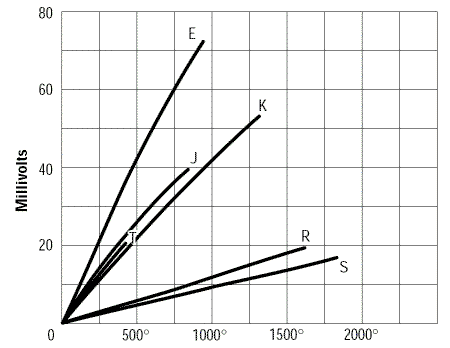
Figure 4. Thermocouple voltage as a function of temperature
| Type | Metal A (+) | Metal B (-) |
| E | Chromel | Constantan |
| J | Iron | Constantan |
| K | Chromel | Alumel |
| R | Platinum | Platinum 13% Rhodium |
| S | Platinum | Platinum 10% Rhodium |
| T | Copper | Constantan |
In order to obtain a better picture of this non-linearity, let’s look at the Seebeck coefficient as a function of temperature:
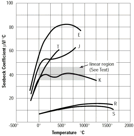
Figure 5. Seebeck coefficient as a function of temperature for different types of thermocouples
Note that the type K thermocouple has a section which is almost linear between 0°C et 1000°C with a Seebeck coefficient α fluctuating around 40 µV/°C. Therefore this type of thermocouple can be used directly with a voltmeter multiplier and reference 0°C to obtain the temperature with moderate accuracy.
Calculation using tables
After reading the voltage value V, for example 8.35687 mV, with a type K thermocouple (Chromel/Alumel), let’s look in the ITS-90 table:
| ITS-90 table for Type K Thermocouple Thermoelectric voltage in mV | |||||||||||
| °C | 0 | 1 | 2 | 3 | 4 | 5 | 6 | 7 | 8 | 9 | 10 |
| 190 | 7.739 | 7.779 | 7.819 | 7.859 | 7.899 | 7.939 | 7.979 | 8.019 | 8.059 | 8.099 | 8.138 |
| 200 | 8.138 | 8.178 | 8.218 | 8.258 | 8.298 | 8.338 | 8.378 | 8.418 | 8.458 | 8.499 | 8.539 |
| 210 | 8.539 | 8.579 | 8.619 | 8.659 | 8.699 | 8.739 | 8.779 | 8.819 | 8.860 | 8.900 | 8.940 |
We can see that this value is between Tinf 205 °C (8.338 mV) and Tsup 206 °C (8.378 mV). Let’s make a calculation by interpolation between the values 205 and 206 °C:
8.35687 – 8.338 = 0.01887 mV (remaining voltage above 205 °C)
8.378 – 8.338 = 0.040 mV for a difference of 1 °C
0.01887 / 0.040 = 0.471 °C in addition
The temperature is therefore 205 + 0.471 = 205.471 °C
In summary, the equation is:
= 205 + [(8.35687 – 8.338) / (8.378 – 8.338)] = 205.471 °C
Or:
$$ T\left( {^\circ C} \right) = {T_{inf}}\left( {^\circ C} \right) + \frac{{V – {V_{inf}}}}{{{V_{sup}} – {V_{inf}}}} $$
Calculation by polynomial equation
It is possible to calculate the temperature from the thermoelectric voltage by means of a polynomial equation:
$$ {T_{90}} = {c_0} + {c_1}V + {c_2}{V^2} + \cdots + {c_n}{V^n} $$
T90 = Temperature in °C
V = Thermoelectric voltage in mV
c = Polynomial coefficients
n = Maximum order of the polynomial equation
| Example of coefficients for type K thermocouples | |||
| Temperature (°C) | -200 to 0 | 0 to 500 | 500 to 1372 |
| Voltage (mV) | -5.891 to 0.000 | 0.000 to 20.644 | 20.644 to 54.886 |
| c0 | 0 | 0.000000E+00 | -1.318058E+02 |
| c1 | 2.5173462E+01 | 2.508355E+01 | 4.830222E+01 |
| c2 | -1.1662878E+00 | 7.860106E-02 | -1.646031E+00 |
| c3 | -1.0833638E+00 | -2.503131E-01 | 5.464731E-02 |
| c4 | -8.9773540E-01 | 8.315270E-02 | -9.650715E-04 |
| c5 | -3.7342377E-01 | -1.228034E-02 | 8.802193E-06 |
| c6 | -8.6632643E-02 | 9.804036E-04 | -3.110810E-08 |
| c7 | -1.0450598E-02 | -4.413030E-05 | 0 |
| c8 | -5.1920577E-04 | 1.057734E-06 | 0 |
| c9 | 0 | -1.052755E-08 | 0 |
| Error (°C) | -0.02 to 0.04 | -0.05 to 0.04 | -0.05 to 0.06 |
| The coefficients for other types of thermocouples are given in appendices at the end of the ITS-90 tables | |||
This is in a sense the reciprocal or converse function of the equation for converting voltage to temperature:
For all types of thermocouples (except K at t>0°C), we have:
$$ V(mV) = \mathop \sum \limits_{i = 0}^n {\left( {{t_{90}}} \right)^i} $$
For type K thermocouples at temperatures above 0°C, we have:
$$ T\left( {^\circ C} \right) = {T_{inf}}\left( {^\circ C} \right) + \frac{{V – {V_{inf}}}}{{{V_{sup}} – {V_{inf}}}} $$
Ci = Coefficients from C0 to Cn
t90 = Temperature of the thermocouple in °C
a0 to a2 = Specific coefficients of exponentiation only for type K thermocouples and temperatures above 0 °C
e= natural logarithm constant: 2.71828…
| Example of coefficients for type K thermocouples | ||
| Temperature (°C) | -270 to 0 | 0 to 1372 |
| c0 | 0 | -0.176004136860e-1 |
| c1 | 0.394501280250e-1 | 0.389212049750e-1 |
| c2 | 0.236223735980e-4 | 0.185587700320e-4 |
| c3 | -0.328589067840e-6 | -0.994575928740e-7 |
| c4 | -0.499048287770e-8 | 0.318409457190e-9 |
| c5 | -0.675090591730e-10 | -0.560728448890e-12 |
| c6 | -0.574103274280e-12 | 0.560750590590e-15 |
| c7 | -0.310888728940e-14 | -0.320207200030e-18 |
| c8 | -0.104516093650e-16 | 0.971511471520e-22 |
| c9 | -0.198892668780e-19 | -0.121047212750e-25 |
| c10 | -0.163226974860e-22 | |
| Exponential coefficients for temperatures above 0 °C | ||
| a0 | 0.1185976 | |
| a1 | -0.1183432e-3 | |
| a2 | 0.1269686e+3 | |
VOLTAGE OF DIFFERENT THERMOCOUPLES FOR A TEMPERATURE OF 350 °C
| Voltage calculated in mV | |||
| Type | By ITS-90 table | Voltage | Difference in % |
| B | 0,596 | 0,596 | -0,018 |
| E | 24,964 | 24,964 | 0,001 |
| J | 19,090 | 19,090 | 0,002 |
| K | 14,293 | 14,293 | 0,001 |
| N | 11,136 | 11,136 | 0,002 |
| R | 2,896 | 2,896 | 0,007 |
| S | 2,786 | 2,786 | -0,008 |
| T | 17,819 | 17,819 | -0,002 |
Over the years, many types of thermocouples have been developed in order to solve measurement problems.
Noble metal
Noble metal thermocouples, types B, R and S, based on platinum or platinum/platinum rhodium thermocouples share similar properties.
Diffusion
The diffusion of metal vapour at high temperatures can change the calibration of the platinum wires; therefore they should only be used inside a non-metallic sheath e.g made from high purity ceramic. An exception to this rule is a platinum sheath, but that is an expensive option.
Stability
Thermocouples based on platinum are by far the most stable of all. The type S is so stable that it is used as a standard for calibrating the temperature between the solidification point of antimony (630.74°C) and that of gold (1064.43°C).
Type B
The type B thermocouple is the only common thermocouple which shows a double evaluation ambiguity.
Non-precious metal thermocouples
In contrast to noble metal thermocouples, non-precious metal thermocouples do not have a precise chemical composition. It is possible to use any combination of metals which give temperature curve results within standard error limits. This results in a number of rather interesting combinations. For example, as we saw above, constantan does not have defined proportions, but is a generic name for copper-nickel alloys.
Type E
The type E thermocouple is suitable for low temperature measurements due to its high Seebeck coefficient (58 µV/°C), low conductivity and corrosion resistance. The Seebeck coefficient for the type E is the highest of all standard thermocouples, which makes it useful for detecting small changes in temperature.
Type J
Iron, the positive element in a type J thermocouple is an inexpensive metal, but one which is rarely very pure. The properties of type J thermocouples may vary due to impurities in the iron. Nevertheless, type J thermocouples are popular due to their high Seebeck coefficient and low cost. A type J thermocouple should never be used above 760°C because of sudden magnetic transformation which can cause decalibration even on return to lower temperatures.
Type T
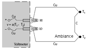
The type T has a copper wire, a significant advantage in the monitoring of temperature differences in that enables two type T thermocouples to be installed in series thus eliminating the need for cold junction compensation.
Types K and N
Type K thermocouples have always been widely used. They are suitable for measuring high temperatures due to their resistance to oxidation. The type N is becoming increasingly popular as a replacement for the type K. The result is slightly below that of the type K (lower Seebeck coefficient), but its resistance to oxidation is even greater. The yield curve of the type N thermocouple depends on the wire gauge and there are two distinct characteristic Nicrosil-Nisil curves depending on the wire gauge.
In the same year that Seebeck discovered thermoelectricity, Humphrey Davy (1778-1829) claimed that the resistivity of metals showed a marked dependence on temperature. Fifty years later, William Siemens used platinum in a resistance thermometer. The propitiousness of this choice has been proved by the use of platinum as the main element in high precision resistance thermometers. In fact, the Platinum Resistance Temperature Detector or PRTD is used today from the triple point of hydrogen (-259.34 °C) to the freezing point of silver (961.78°C). Platinum is particularly suitable as it can withstand a wide range of temperatures while remaining highly stable and suffering almost no deterioration.
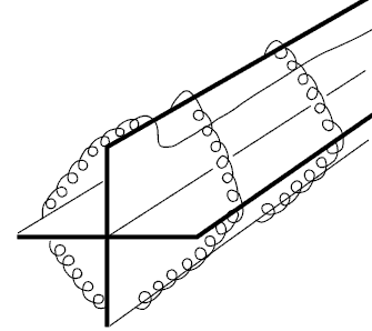
In 1932, C.H. Meyers proposed building a resistance temperature detector (RTD) comprising a platinum wire wound in a helix round a cross-shaped mica support, all encased in a glass tube. This system minimises the tension on the wire while maximising the resistance. Although this construction produces a highly stable element, the quality of the thermal contact between the platinum and the point to be measured is poor and consequently the thermal response time is slow. The fragility of the structure restricts its use today to that of a laboratory instrument.
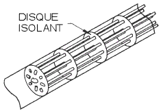
A different laboratory instrument has replaced Meyer’s design. This is the “birdcage structure proposed by Evans and Burns. The constraints on resistance caused by the time and temperature are thus minimised and the “birdcage” became the norm in the laboratory. Its fragile structure and sensitivity to vibrations mean that it is not suitable for industrial environments.
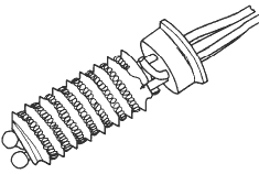
More robust construction techniques are shown in the figures opposite: a bifilar platinum wire is wound round a glass or ceramic coil. The bifilar winding reduces the magnetic induction and associated noise. Once the wire has been wound round the coil, the structure is sealed with molten glass. Unless the coefficients of expansion of the platinum and the coil are perfectly matched, expansion of the wire will result in a change in resistance with the consequence of a possible permanent change in the resistance of the wire.

There are RTD versions which offer a compromise between the birdcage and the sealed spiral. This approach uses a helicoidal platinum spiral wound round a ceramic cylinder and held in place by sintered glass.

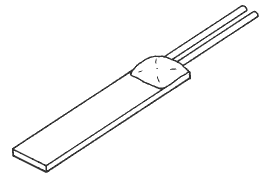
Modern manufacturing techniques use a platinum or metal film on a flat, etched ceramic substrate, guided by laser and sealed. The film RTD offers a significant reduction in assembly time and has the advantage of increased resistance for a given size. The manufacturing technology means that the devices are small with low thermal inertia; they can respond rapidly to changes in temperature.

Film RTDs are slightly less stable than wire RTDs but the benefits in terms of size, production cost and ease of use mean that they are very widely used.
All metals produce a positive change in resistance in response to a positive change in temperature, which is the main function of an RTD. System error is minimised where the RTD’s resistance nominal value is large; this means using a metal wire with high resistivity.
| Resistivity of the metals used in RTDs | ||||
| Metal | Symbol | Resistivity Ω·cm/f | Resistivity Ω·mm²/m | Resistivity siemens |
| Gold | Au | 13 | 2,1612e-2 | 4,6272e+7 |
| Silver | Ag | 8,8 | 1,4629e-2 | 6,8356e+7 |
| Copper | Cu | 9,26 | 1,5394e-2 | 6,496e+7 |
| Platinum | Pt | 59 | 9,8083e-2 | 1,0195e+7 |
| Tungsten | W | 30 | 4,9873e-2 | 2,0051e+7 |
| Nickel | Ni | 36 | 5,9847e-2 | 1,6709e+7 |
Due to their low resistivity, gold and silver are rarely used in RTDs.
Le tungstène a une résistivité relativement élevée, mais est réservé pour des applications à très hautes températures parce qu’il est extrêmement fragile et difficile à travailler.
Tungsten has a relatively high resistivity, but is reserved for applications at very high temperatures because it is extremely fragile and difficult to work. Its upper temperature limit is only around 120 °C.
The most common RTDs are made of platinum, nickel or nickel alloys. Wires in nickel alloy are economic and used in a restricted temperature range, but they are non-linear and tend to drift over time.
Platinum is the obvious choice for all measurements.
The common RTD resistance values extend from 10 ohms for the birdcage model to several thousand ohms for metal film RTDs. The most common value is 100 ohms at 0 °C, called the R0 coefficient. These RTDs are called Pt 100s.
The DIN 43760 standardised temperature coefficient of platinum wire is: α = 0.00385. For a resistance of 100 ohms at 0 °C, this corresponds to + 0.385 ohm per °C (European α). α is therefore the average slope from 0°C to 100°C $$ \alpha = \frac{{{R_{100}} – {R_0}}}{{ {R_0} \times 100^\circ C.}} $$. There is a wide range of RTDs which have different α coefficients and ohm values at 0°C detailed in their technical properties. The most commonly used RTD is that with an α coefficient of 0.00385 and ohm value at 0°C of 100 Ω. It is known as Pt100.
| Values of some RTDs | ||
| R at 0°C (Ω) | α (Ω/Ω/°C) | Average sensitivity (Ω/°C) |
| 25.5 | 0.00392 | 0.1 |
| 100 | 0.00392 | 0.392 |
| 100 | 0.00391 | 0.391 |
| 100 | 0.00385 | 0.385 |
| 200 | 0.00385 | 0.770 |
| 470 | 0.00392 | 1.845 |
| 500 | 0.00392 | 1.963 |
| 500 | 0.00391 | 1.955 |
| 500 | 0.00385 | 1.925 |
| 1000 | 0.00385 | 3.850 |
| 1000 | 0.00375 | 3.750 |
| 10000 | 0.00385 | 38.50 |
| International standards DIN 43760 (IEC 751, BS-1904, JIS C1604) | ||
| Parameter | Class A | Class B |
| R0 | 100Ω ±0,06% | 100Ω ±0,12% |
| Alpha, α | 0,00385 ±0,000063 | 0,00385 ±0,000063 |
| Range | -200°C to 650°C | -200°c to 850°C |
| Res, RT | ±(.06+.0008|T|-2e-7T2) | ±(.12+.0019|T|-6e-7T2) |
| Temp, T | ±(0.3+0.002|T|)°C | ±(0.3+0.005|T|)°C |
The choice of connection method and electronic interface depends on the measurement accuracy required.
3 connection modes can be used for an RTD: 2-wire, 3-wire or 4-wire.
2-Wire measurements
This is the simplest method but results in an error proportional to the length of the cable used for the connection. A standard AWG24 cable (85 Ω/km) introduces an error of the order of 0.42°C per metre of connection for an RTD Pt100 sensor.

The slope and the absolute value are small numbers, especially if we take into account the fact that the measurement wires connected to the sensor can be of several ohms or even tens of ohms. A small wire impedance can contribute to a significant error in our temperature measurement. A wire impedance of 10 ohms results in an error of 10/0.385 or approximately 26°C in this case.

One way of avoiding this problem is to use a measuring device with a bridge. Measurement via a bridge, in this case a Wheatstone bridge, is an indirect indication of the resistance of the RTD. The bridge requires four connection wires, an external source and three resistors which have a temperature coefficient of zero.

3-Wire measurements
The “3-wire” method very often provides a measurement of sufficient quality for the majority of industrial applications. It is based on the hypothesis of equal resistance of the 3 wires. Use of an AWG18 cable (21 Ω/km) introduces an error of less than 0.4°C per 100 m of connection


In order to avoid subjecting the three resistors of the bridge to the same temperature as the RTD, the latter is separated from the bridge by a pair of connecting wires. These wires recreate the problem we saw above: the impedance of the connecting wires affects the temperature reading. This effect can be minimised by using a three-wire bridge configuration. If wires A and B are the same length their impedance effects will cancel each other out because each is in an opposite part of the bridge. The third wire C acts as measuring device in which no current is circulating. The Wheatstone bridge shown in figure 41 creates a non-linear relationship between the change in resistance and the change in the measurement voltage of the bridge. This requires an additional equation to convert the measurement voltage of the bridge into equivalent impedance of the RTD.

4-Wire measurements
This assembly offers the greatest accuracy, as the voltage is measured on the active part of the sensor with a high impedance electronic interface. The resistance of the connection cables no longer affects the measurement error.

The best technique is to use a known source of current and to measure the voltage at the RTD terminals remotely. As no current is circulating in the voltage measurement wires, there is no drop in voltage and therefore no resistance measurement error. The voltage read on the voltmeter is directly proportional to the resistance value of the RTD. The three resistors of the bridge are replaced by a reference resistor enabling the current generated to be accurately established (figure 42). The disadvantage is the need for an additional wire compared with the 3-wire bridge. This is a small price to pay in order to obtain an accurate measurement of the resistance.

Pt100 sensors (platinum 100 Ω (PRTD)) are more linear than thermocouples:

Figure 6 Change in the coefficient of linearity of a type S TC and a Pt100
Figure 6 Change in the coefficient of linearity of a type S TC and a Pt100 The relationship between the temperature and the ohm value of the RTDs was calculated by Callendar, then later refined by Van Dusen, which is why it is known as the Callendar-Van Dusen (CVD) equation.
$$ {R_T} = {R_0} + {R_0}\alpha \left[ {T – \delta \left( {\frac{T}{{100}} – 1} \right)\left( {\frac{T}{{100}}} \right) – \beta \left( {\frac{T}{{100}} – 1} \right)\left( {\frac{{{T^3}}}{{100}}} \right)} \right] $$
Where RT = resistance at T°C, R0 = resistance at 0°C, α = temperature coefficient at 0°C in Ω/Ω/°C, δ = coefficient of linearisation, β = second coefficient of linearisation for negative temperature values (β = 0 for T > 0°C).
This equation has been converted to enable it to be used more easily with the coefficients A, B and C given by the standard DIN 43760 (IEC 751) and the data sheets of the components:
$$ {R_T} = {R_0}\left[ {1 + AT + B{T^2} – C\left( {T – 100} \right){T^3}} \right] $$
C=0 for T>0°C.
| Coefficients for different α values | |||
| Coefficient | Value | Value | Value |
| α | 0,003850 | 0,003926 | 0,003911 |
| δ | 1,4999 | ||
| β | 0,10863 | ||
| A | 3,9083e-3 | 3,9848e-3 | 3,9692e-3 |
| B | -5,775e-7 | -5,870e-7 | -5,8495e-7 |
| C | -4,18301e-12 | -4,000e-12 | -4,2325e-12 |
These three α values represent the three main specifications for RTDs.
- 0.03850 Ω/Ω/°C: Standards DIN 43760, IEC 751 and other international specifications, called the European Standard.
- 0.003926 Ω/Ω/°C: Requires platinum of 99.999% purity or better, called the American Standard.
- 0.3911 Ω/Ω/°C: Often called the US Industrial Standard.
The CVD equation calculates resistance as a function of temperature; this is the converse of the most common applications: temperature as a function of resistance. In order to convert the RTD resistance into temperature, we need to use a 2nd degree quadratic equation, which is in a sense the reciprocal of the CVD equation but only for temperatures above 0°C:
$$ T = \frac{{ – A + \sqrt {{A^2} – 4B\left( {1 – \frac{{{R_T}}}{{{R_0}}}} \right)} }}{{2B}} $$
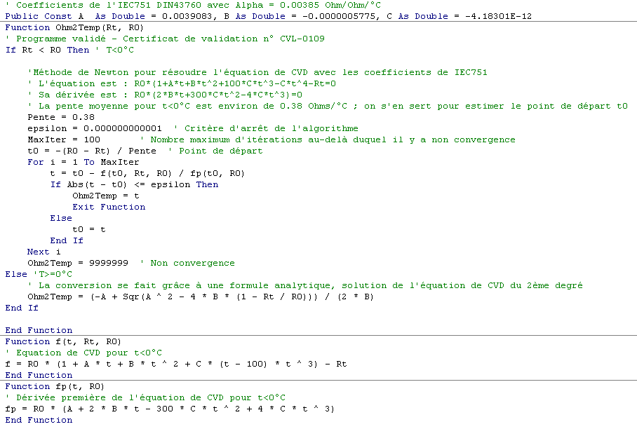
For temperatures below 0°C, the CVD equation is too complex to solve, and it is necessary to use numerical methods. The most accurate is to find the root of the CVD equation numerically; in other words, to solve the following equation:
$$ f\left( T \right) = {R_0}\left[ {1 + AT + B{T^2} + C\left( {T – 100} \right){T^3}} \right] – {R_T} = 0 $$
The most appropriate method is the tangent method (or Newton’s algorithm). This method has the advantage of converging with certainty provided that the root is within the given interval, which is achievable knowing the average sensitivity of an RTD. This method also requires knowing the derivative of the CVD equation which can easily be calculated:
$$ \frac{{df\left( T \right)}}{{dT}} = {R_0}\left[ {A + 2BT + 4C{T^3} – 300C{T^2}} \right] $$
Finally, it is necessary to be certain that the equation has only one root, which is the case with the CVD equation. The algorithm, simple, can be found in all books on numerical methods. It consists in determining for a starting point $$ {{t_0}} $$, the tangent at this point $$ f’\left( {{t_0}} \right) $$ which intersects with the curve at a new point $$ {{t_1}} $$. At this point, we recalculate the tangent $$ f’\left( {{t_1}} \right) $$ which in turn intersects with the curve at a point $$ {{t_2}} $$, etc… until the gap between two successive points is smaller than the stopping criterion (defined by ε). The program “RTD.xls” uses this algorithm. Here is the source code:
Resistance thermometer systems are susceptible to three types of errors:
- The tolerances inherent in the resistance itself
- The temperature gradients between the thermometer and the medium to be measured
- The errors and defects in the connection between the sensor and the measuring instrument.
Some sources of error are electric; others result from the mechanical construction of the thermometer. Potential sources of error include interchangeability and conformity. Conformity indicates the extent to which deviation from the standard curve is permissible. Conformity has two components: a tolerance at the reference temperature, normally 0°C, and a tolerance on the slope.
These possible deviations are defined in the standards. For example, the standard DIN 43760 class B requires calibration at less than 0.12Ω (0.3°C) at 0°C, but allows the curve to deviate from the nominal 0.00385 by ±0.000012 Ω/Ω/°C. This can give deviation of 0.8°C at 100°C, 1.3°C at 200°C, and up to 3.8°C at 700°C.
It is, therefore, important to know precisely the tolerances applicable to the system used.
A resistance thermometer is a passive probe; it requires the passage of a measuring current in order to produce a useful signal. This measuring current heats the element and raises its temperature. Errors will result unless the additional heat is absorbed.
In order to evaluate the measurement error as a function of the current injected through the resistive element, the self-heating coefficient has been defined. The units of the self-heating coefficient are °C/W. As a first approximation, the temperature measurement error is inversely proportional to the power injected into the resistor. Electrical power is calculated according to the following formula: P = R*I². The greater this coefficient, the greater the measurement error for a given current and experimental conditions.
To reduce the error due to this effect, under given conditions, we generally try to reduce the measurement current, but we can’t avoid it. As mentioned above, operating conditions can strongly influence this phenomenon. When temperature measurements are made on a moving fluid, this coefficient decreases with fluid flow speed, as the fluid carries away more and more heat.
From a normative point of view, the IEC60751 standard prescribes the conditions for evaluating this phenomenon. According to this standard, this phenomenon can be quantitatively evaluated in an air stream or in a water stream. In air, the temperature must be between 0 and 30°C, with an air speed of (3 +/- 0.3) m/s. In water, the velocity must be greater than 0.2 m/s. A probe based on a platinum resistive element must not have an error due to self-heating greater than 25% of the standard tolerance class. In practice, the measurement current for Pt100 probes (100 Ohm resistance at 0°C) rarely exceeds 1 mA. As an example, we’ll take a self-heating coefficient value of 20°C/W. For a current of 1 mA and a temperature of 0°C, the power injected into the resistor is [ R*I² = 100 * 1/1000 * 1/1000 * Ω * A * A = 10-4 W ]. This corresponds to a temperature rise of 0.002°C. If the measurement current is 5 mA, the power would be 2.5*10-3 W and the temperature change due to this current would be 0.05 °C.
NB, the resulting error is inversely proportional to the capacity of the thermometer to dispose of the additional heat; this depends on the thermometer materials, construction and environment.
The worst case occurs when a high-value resistor is in a small body. Film RTDs, with little surface area to absorb heat, are a case in point.
Self-heating also depends on the medium in which the thermometer is immersed. The error in still air can be 100 times greater than in moving water.
A time constant which indicates the response of a thermometer to a change in temperature. A common expression is the time a thermometer takes to reflect 63.2% of a temperature graduation in moving water. A 90% change is referred to as “T90”.
The speed of response depends on the mass of the thermometer and the rate of heat transfer between the external surface of the element and the medium in which it is immersed. A small time constant reduces errors in a system subject to rapid changes in temperature.
Measuring a quantity means comparing it to a quantity of the same type taken as a reference. This latter quantity constitutes a unit of measurement; the set of legal units of measurement constitute a system known as the Système International (SI).
In metrology, the science of measurement, the term measure or measurement has a number of meanings which it is worth noting here; it may refer to:
- a value: the measurement of a distance is 100 metres
- a result: measurement to within 1%
- an action: making a measurement of electric power
- an instrument: a capacity measure
To avoid ambiguity, it is preferable to refer to the value of a quantity, the result of a measurement, measuring and measuring equipment. However, where there is no possibility of confusion, a measurement refers to the result of measuring.
A standard is a measuring instrument designed to define or represent, preserve or reproduce a unit of measurement of a quantity (or a multiple or submultiple of such a unit).
Various type of standard are produced, depending on how they are used. In the case of a given quantity, the primary standard is the highest quality in terms of measurement; it is never used directly for measurement except for comparison with secondary standards. Working standards used to check measuring instruments are produced from a secondary standard.
A measurement error is the discrepancy between the result of a measurement and the value of the quantity measured.
This value may be the true value or, if this is not known (as is most often the case), the conventionally accepted true value of the quantity, or alternatively the arithmetic average of the results of a series of measurements. This discrepancy can have various causes and in general only an upper limit can be determined, referred to as measurement uncertainty.
This is an error that remains constant in absolute value and sign when several measurements of the same fixed quantity are made under the same conditions.
The causes of systematic errors may or may not be known. If such an error can be determined by calculation or experiment, an appropriate correction is applied to the measurement result. If a systematic error cannot be determined but if it can be assumed to be sufficiently small by comparison with the imprecision of measurement, it is assessed approximately and taken into account in the calculation of the error.
Example of a systematic error: measurement of a mass using a supposed 1kg test weight, where the true mass is 1.005 kg.
This is an error that varies unpredictably in absolute value and sign when a large number of measurements of the same quantity are made under virtually identical conditions. It is not possible to take a chance error into account by applying a correction to the raw measurement result. It is only possible to fix an upper limit for such an error at the end of a series of measurements. A chance error is often called an accidental error or random error.
This is an often gross error resulting from mismeasurement. For example, it may be due to misreading or to a defective instrument or even incorrect use of an instrument. It is not taken into account in the analysis of measurements.
A number of errors may be committed when a measurement is made: error due to the measuring instrument, error due to accessories of the measuring instrument, reading error, etc. These are called partial errors. Measurement uncertainty must enable all partial errors to be taken into account by combining them in accordance with a law under which twice the square root of the sum of the squares of the partial errors is applied to the measurement result.
This is the difference between the result of measurement X and the comparison value which may be the true or conventionally true value Xv, or the arithmetic average x of the results of a series of measurements. In the first case, the absolute error is said to be actual (dx = X – Xv); in the second case it is said to be apparent (dx = X – x).
This is the quotient of the absolute error and the comparison value used to calculate the absolute error (dx/Xv or dx/x).
In the case of a series of n measurements of the same quantity, the dispersion of the results obtained around the mean is characterised by the average quadratic deviation σ which is given by the following formula:
$$ \sigma = \sqrt {\frac{{\mathop \sum \nolimits_{i = 1}^n {{\left( {{x_i} – \bar x} \right)}^2}}}{{n – 1}}} $$
In the case of a large numbers of measurement, the result of measurement number i (i = 1,2,3,…,n) is designated by $$ \bar x $$ and the average $$ \bar x = \frac{{\mathop \sum \nolimits_{i = 1}^n {x_i}}}{n} $$.
Increasing the number of measurements decreases the significance of chance errors and an average of the results can be accepted as the result of a series of measurements.
The “GUM” (Guide to Uncertainty in Measurements) however recommends weighting this standard deviation by a coefficient, known as the “Student’s”, symbol s, if the number of measurements is less than or equal to 5.
- For 3 measurements, s=9.2
- For 4 measurements, s=6.6
- For 5 measurements, s=5.5
Thus, the standard deviation formula becomes:
$$ \sigma = \frac{s}{{3\sqrt n }}\sqrt {\frac{{\mathop \sum \nolimits_{i = 1}^n {{\left( {{x_i} – \bar x} \right)}^2}}}{{n – 1}}} $$
Be careful not to confuse the standard deviation with the spread which is the difference between the minimum and maximum values of the quantities measured: $$ e = {x_{max}} – {x_{min}} $$.
The main basic errors in the case of an electromechanical instrument are due to friction between moving components and fixed elements, mechanical inertia, thermal inertia, reading errors, in particular a parallax error (if the pointer is some distance from the surface of the scale and the reader cannot position himself face-on to the surface).
In the case of high-quality instruments, the manufacturer supplies a calibration curve: this shows the relationship between the values of the quantity measured and the values shown by the instrument. If necessary, correction curves may be applied to correct the results if one or more material quantities are outside the reference conditions.
A number of factors are to be considered when assessing a measuring instrument.
Trueness characterises the ability of an instrument to give results equal to the true value of the quantity measured, i.e. not marred by systematic errors.
Fidelity characterises the ability of an instrument to give consistent results, i.e. not marred by chance errors for the same measured quantity.
Sensitivity means the smallest amount dx that can be measured in the case of a certain value x of the quantity measured. The sensitivity may be constant along the length of the scale. Note that the lower dx is, the greater the sensitivity.
Hysteresis or reversibility characterises the ability of an instrument to give the same result when the same value for the quantity measured is obtained by increasing values or decreasing values.
The response time of an instrument is the time that elapses between an abrupt change in the quantity to be measured and the point at which the instrument gives a definitive reading of the new value of the quantity.
The precision of an instrument is equal to the ratio dx/x of the overall error dx and the value x of the quantity to be measured. It characterises the quality of an instrument from the point of view of errors; the closer the results are to the true value, the greater the precision (i.e. dx is small).
The resolution, used for instruments with a digital display, refers to the smallest value that can be displayed. Not to be confused with the sensitivity or precision.
The measurement range is the set of values for which the results obtained are not marred by an error greater that the maximum permitted error. Some instruments may have several measurement ranges.
The rating of an instrument is the value of the quantity to be measured which corresponds to the upper limit of the measurement range. For example, in the case of an ammeter, if this upper limit is 5 A, its rating is said to be 5 A.
A measuring instrument (and its accessories) are characterised by a number known as the class index. This represents the upper limit of the absolute intrinsic error (i.e. due to the instrument alone used under reference conditions) expressed in hundredths of the largest reading that the instrument can give.
Thus, for example, an ammeter of class 0.2 is an instrument for which the absolute intrinsic error does not exceed 0.2% of its largest reading, when used in normal conditions. If this ammeter has 100 divisions, this absolute intrinsic error is thus equal to or less than 0.2/100*100=0.2 of a division.
In the case of an instrument with several ratings, the result remains the same whatever the rating; in contrast the expression of this error in amperes changes with the rating since 0.2 of a division in a scale of 100 divisions represents 0.2/100 of the rated capacity (0.002 A for 1 A rating); (0.01 for 5 A rating).
The values of the class indices are established in the standard NF C 42-100. Instruments with the same class index are said to be of the same precision class. Instruments in class 0.1 or 0.2 are designated as standards; those in class 0.5 are laboratory instruments. Instruments in class 1.5 or 2.5 are control instruments.
Rounding a decimal number means assigning it the value closest to the required precision. Depending on the level of rounding required, look at the figures immediately after:
- if it is 0; 1; 2; 3 or 4 the rounded number remains unchanged
- If it is 5; 6; 7; 8 or 9 the rounded number is increased by 1
Examples:
0.9273426 ➨ 0.927343 ; 0.9 ➨ 1 ; 2.5 ➨ 3 ; 1.34 ➨ 1.3