How is the voltage produced by a thermocouple measured?

Now that we know that a thermocouple generates a voltage the magnitude of which is a function of the temperature and the Seebeck coefficient (α) of the junction of the two dissimilar metals, all that remains is to measure this using a voltmeter and then calculate the temperature from the voltage measured.

Connection to a voltmeter

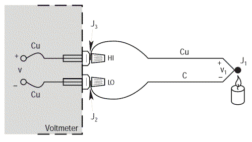
Let’s connect a Copper/Constantan thermocouple (Type T) to the terminals of a voltmeter and making the calculation using α = 38.75µV/°C, we obtain a temperature figure which is independent of the environment around the thermocouple.

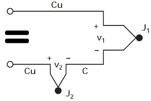
Finally, by referring to the equivalence diagram (=), the resulting voltage measured by the voltmeter is equal to V1 – V2, i.e. It is proportional to the temperature difference between J1 and J2.

We can only find the temperature of J1 if we know that of J2.

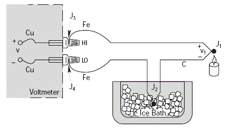
Reference to the external junction

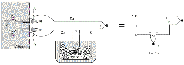
A simple way of the determining the temperature of junction J2 accurately and easily is to immerse it in a bath of melting ice which forces its temperature to 0°C (273.15 K). J2 can then be taken as the reference junction. Thus there is now a reference value of 0°C at J2.

And using a different type of thermocouple?

The previous examples used a Copper/Constantan thermocouple (Type T) which is simple to use for demonstrations as the voltmeter terminals are also made of copper and this only induces a single parasitic junction. Let’s go through the same example with an Iron/Constantan thermocouple (Type J) instead of Copper/Constantan.

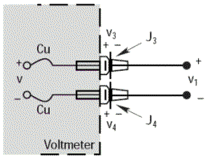
The voltmeter will show a voltage V equal to V1 only if the thermoelectric voltages V3 and V4 are identical, since they are in opposition; i.e. if the parasitic junctions J3 and J4 are at the same temperature.

It is essential that the voltmeter connection terminals are at the same temperature in order to prevent any drift in the measurement.

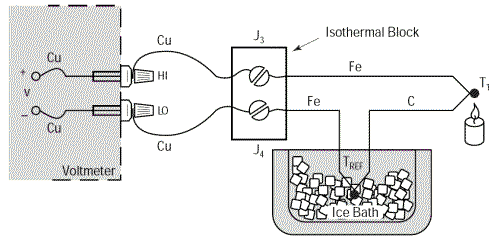
This problem can be eliminated by extending the copper wires so that they are only connected as close as possible to the thermocouple using an isothermal junction block. This type of block is an electrical insulator but a good heat conductor such that it keeps junctions J3 and J4 permanently at an identical temperature. By proceeding thus we can very easily move the thermocouple away from the measuring instrument without causing problems. The temperature of the isothermal block is irrelevant as the thermoelectric voltages at the two Cu-Fe junctions are in opposition.

We will still have: V = α(TJ1 – TREF)

Eliminating the bath of melting ice

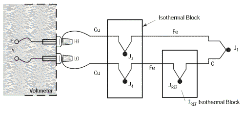
The circuit described above enables us to take accurate, reliable measurements away from the thermocouple, but how useful it would be to eliminate the need for the bath of melting ice. Let’s begin by replacing the bath of melting ice with another isothermal block which will be kept at the temperature TREF.

Since we have already seen that the temperature of the isothermal block supporting junctions J3 and J4 is not relevant – provided that these two junctions are at the same temperature – there is no reason not to combine the two blocks into one which will be kept at the temperature TREF.

We will still have: V = α(TJ1 – TREF)

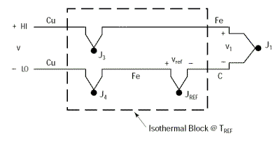
However, this new circuit has the disadvantage that it requires two thermocouples to be connected. We can happily eliminate the additional thermocouple by combining the junctions Cu-Fe (J4) and Fe-C (JREF). This is possible due to the law of intermediate metals. This empirical law states that a third metal (in this case Iron) inserted between the two different metals in a thermocouple does not affect the voltage generated provided that the two junctions formed by the additional metals are at the same temperature.

This results in the equivalent circuit below where our two junctions J3 and J4 become the Reference junction for which the relationship: V = α(TJ1 – TREF) remains valid.

Summary

We have in sequence:

1. Created a Reference junction,
2. Shown that V = α(TJ1 – TREF),
3. Put the Reference Junction into a bath of melting ice,
4. Eliminated the problem with the voltmeter terminals,
5. Combined the reference circuit,
6. Eliminated the bath of melting ice

to arrive at a simple circuit, which is easy to use, reliable and highly effective. However, we need to know the exact temperature TREF of the isothermal junction block in order to apply the relationship: V = α(TJ1 – TREF) and thus be able to calculate the temperature at the junction J1 which remains our objective. Therefore we need to establish the temperature of the isothermal block which we will do using the RT device. Using a multimeter, we can:

1. Measure RT in order to calculate TREF
2. TREF to an equivalent junction voltage VREF
3. Measure V and add VREF to obtain V1
4. Convert V1 to temperature TJ1

Proceeding in this way is called Software Compensation because it uses calculation to compensate for the fact that the cold junction (or reference junction) is not at zero degrees. The temperature detector for the isothermal block can be any device which has a property proportional to the absolute temperature: an RTD (Resistance Temperature Detector), a Thermistor or an integrated sensor.